Huw Dixon

The Generalized Taylor Economy (GTE)

A Generalized Taylor Economy (GTE) is one where there are many sectors: within each sector there are contracts of a particular duration, and these operate according to Taylor's (1980) staggered contracts model. So, if the longest duration of contracts is \(F\) periods, there will be up to F sectors \(i=1 \ldots F\). In sector\(i\), all contracts (price-spells) last for \(i\) periods, and each period a proportion of \(\frac{1}{i}\) prices will be reset. The share of each sector is \(\alpha_i \ge 0\), with \(\sum_{i=1 \ldots F}\alpha_i = 1\)

A simple Taylor economy is simply one where only one sector has a strictly positive share of the prices: \(\alpha_F=1\). For example, in a Taylor 2 economy: \(\alpha_1=0,\alpha_2=1\). In a GTE, there are many sectors with strictly positive shares. We can think of these “sectors” as duration sectors. For example, a firm might set a price for one period and then for four periods. This firm would then move between the \(i=1\) sector and the \(i=4\) sector. The key point is the Taylor assumption that when they set their price, firms know how long it is going to last.

The great advantage of the GTE is that the sector shares can be chosen to reflect any possible distribution of durations: indeed, it can be exactly calibrated to match the empirical distribution. Furthermore, when it is plugged into a macroeconomic model it also gives nice inflation dynamics, particularly for inflation: the response of inflation to monetary policy follows a nice hump shape. Hence the GTE provides a way of getting good dynamics that is consistent with the microdata on prices and/or wages. This contrasts with many existing models which are either inconsistent with the microdata on prices or do not give nice inflation dynamics.

The appropriate distribution corresponding to the GTE is derived in general by Dixon (2012), and earlier versions.   My own inspiration for starting research on the GTE was the following quote from John Taylor (which Engin Kara and I put at the start of our first paper on the GTE):

"There is a great deal of heterogeneity in wage and price setting. In fact, the data suggest that there is as much a difference between the average lengths of different types of price setting arrangements, or between the average lengths of different types of wage setting arrangements, as there is between wage setting and price setting. Grocery prices change much more frequently than magazine prices – frozen orange juice prices change every two weeks, while magazine prices change every three years! Wages in some industries change once per year on average, while others change per quarter and others once every two years. One might hope that a model with homogenous representative price or wage setting would be a good approximation to this more complex world, but most likely some degree of heterogeneity will be required to describe reality accurately."

John B Taylor, (1999) Staggered Wage and Price Setting in Macroeconomics in: J.B.Taylor and M.Woodford, eds, Handbook of Macroeconomics, Vol. 1, North-Holland, Amsterdam.

¹ These are the first verifiable publication that is available on the web.  Of course, many of these working papers and mimeos will have been presented at conferences in earlier versions. These papers also exist in many different versions: look up the authors in RePEc for the full listing.

If anyone has more papers not included in this listing, please contact me at dixonh@cardiff.ac.uk

Estimated GTEs using Macrodata

Taylor (1994): Estimated using Maximum Likelihood for US data 1961:4–1977:4. Source: Table 2-1, Page 47.

Coenen at al (2007), Table 1 page 2455. US data 1983-2003, German data 1975– 1998.

Carvalho and Dam (2010).  These are first three columns the “empirical distributions” from Table 2 (derived from micro data) and the second three the ex post means from Tables 3-5 using Bayesian estimation using macro-data (1977-2007).

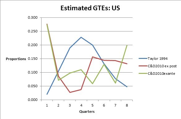
I have not put up the Coenen et al estimated GTE, because the quarter 4 proportion is so large. The Coenen et al and C&D agree that there is a large proportion (27%) of “flexible” prices that can change every quarter, whilst the proportion is just 2% for Taylor (wages).  After that they also differ substantially.  The Taylor peaks at 3-5 quarters (about 20% each), whilst C&D trough at 3-4 quarters.  The C&D ex post has a very fat tail for quarters 5-8, with small proportions (less than 10%) for quarters 2-4.  The C&D ex ante has large ends in quarters 1 and 8, with quarters 2-7 bouncing around 10%.  Taylor dies away after 5 quarters.

Coenen et al come up with some other estimates for the GTE under alternative assumptions about the macroeconomic model: these vary. We have just reported the benchmark here.

Estimates from the Microdata.

I have used a few methods.

Method 1. Use frequency data and assume a Calvo distribution.

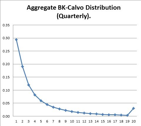
When Engin and I were first formulating the GTE in 2002, we had no data except for Taylor’s distribution which we called “Taylors US economy” which we used in early versions of our GTE paper.  However, there was the price-stickiness table on Pete Klenow’s web-site with the frequency data for 350 CPI categories.  We constructed a possible macroeconomics distribution using the formula for the cross-sectional Calvo distribution we had derived in ECB working paper 489 and which was published in Dixon and Kara JMCB 2006.

This distribution has a long flat tail.  There are 14% with 9 quarters and over.  As we showed in Dixon and Kara (2011), this long-tail can have a disproportionate effect on the way nominal prices respond in the whole economy.

This method is quite simple and can be done with any frequency data at any level of aggregation.  As Dixon and Tian (2012) show, for the UK case at least, this is a good approximation: with highly disaggregated frequency data, the mean and median of the artificial Calvo distribution can equal the actual one.  The main differences between the true distribution and the artificial Calvo are (a) there are more flexible prices in the data than in the Calvo, and (b) there is no 12 month peak in the artificial Calvo.  However, since DSGE models use quarterly data, the differences are to some extent “smoothed out” and as a result the differences between the true data and the artificial Calvo may not matter that much (Dixon and Tian (2012)).

Method 2.  Use the micro-price data (e.g. CPI, PPI).

Method 1 has a weakness: from the frequency there are many possible distributions consistent with a given frequency.   To get the actual Distribution you need access to a microdata set such as the CPI.   The best way to estimate it is to estimate the Hazard function:  as Gabriel and Reiff (2008) showed, this is a robust way to deal with censoring. I have used this in Dixon and Le Bihan (2012), Dixon and Tian (2012) and Dixon (2012).  The hazard function\(h(i)\) gives the probability that a price spell ends after \(i\) periods. The converse concept is the survivor function \(S(i)\), that gives the probability that a price spell will last at least \(i\) periods.

If we assume that there is a steady-state, then there are a series of identities that link together the distributions of durations: in particular the hazard function is related to the cross-sectional distribution of completed spell lengths by the following identity:

\[\alpha_i = i.\bar{h}.h\left(i\right).S\left(i\right),\]

where \(\bar{h}\) is the proportion of firms changing price each period – in Dixon 2012 it is shown that \(\bar{h} = \left(\sum^F_{i=1}S\left(i\right)\right)^{-1}\).

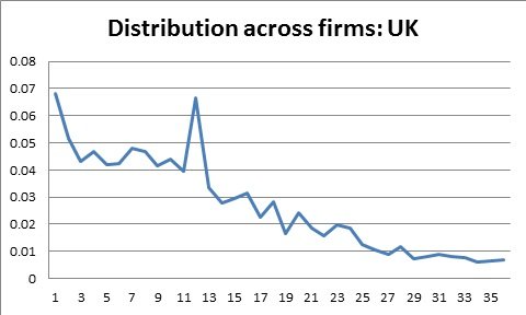
The above gives the distribution derived from the UK data using the Hazard function in Dixon (2012).  The horizontal axis is months, the vertical the share for each month (we only show up to 36 months). As we can see, there is a 12 month “peak” and in general the distribution is declining.  However, there is a fat tail of prices that change very infrequently.

Appendix: Taylor's US economy

Taylor effectively estimated the age distribution, from which he derived the DAF. For completeness, I report the full table with the corresponding hazard and survivor function along with the distribution of durations.  This table (with different notation) first appeared in Dixon (2006), example 5, page 19.